Path-tracing a 3D Chessboard

https://www.youtube.com/watch?v=XyfbU06YFOg

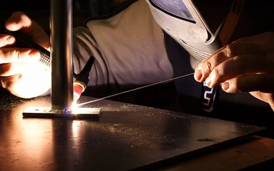
I played chess in college, but stopped when I started working as a programmer. I spent three decades writing graphics and rendering code at PDI DreamWorks and NVIDIA. Now I’m coding an online 3D chessboard you can play on a web page to help reignite my interest in chess and rendering. The goal of the app is to make playing chess on the computer as close as possible to playing at a cafe in real life. My hope is that will help with over-the-board practice, and allow me to create interesting visualizations of tactical elements while adding a bit of fun.

To make the game feel like real life, I wanted photo-realism, and that meant full path tracing. Ray tracing normally just sends a single reflection ray, to get "mirror" reflections, while path tracing sends hundreds of rays for every pixel for more realistic lighting. I wanted it to mimic an outdoor cafe, which is primarily lit by an environment map. I wanted soft reflections and proper shadowing. Since we intended to use an environment map (the blurry background) that meant we needed to shadow properly in all directions, not just, say, to a set of positional or directional light sources using shadow maps, a more traditional GPU approximation. I wanted full global illumination in real time, realistically simulating how light bounces around between surfaces.

In 2025 top-tier AAA games have some ray tracing, even some path tracing, but, as far as I know, none of them use a full real-time path tracer as in film VFX. Not Unreal. Not Unity. They are limited because most GPUs are not powerful enough to rely on full path tracing, and they are committed to rendering a similar look across a wide range of devices.

Even on my high-end NVIDIA 4090 RTX, I barely have enough power to make this scene work at 60 fps, tracing between 6-16 paths per pixel depending on the output resolution. It would be interesting to port the game to a platform, like Vulkan, with support for the latest GPU RTX instructions. I would not be surprised if it was 5-10x faster, though on fewer systems.

I’ll talk more about the design of this game, how it integrates into Lichess.org and with Stockfish, and a bit more of its history in a future blog post. The rest of this post will get into the nitty gritty technical details of the rendering algorithm, with lots of helpful links.

GBuffer > SSGI > SVGF > ACES

Ray tracers spend all their time finding intersections with geometry. Most expect the geometry to be defined by polygons or surfaces, and they build 3D acceleration structures, like K-D trees, that allow them to intersect a ray with the simpler acceleration structure before doing the final intersection test on triangles. The acceleration structure must also deal with moving geometry, and either must be rebuilt or adjusted each frame. Modern GPUs and drivers handle building these acceleration structures for you when you use the native ray-tracing instructions. These days, the acceleration structure is built on the GPU in parallel, often from scratch every frame, even with millions of polygons. Amazing.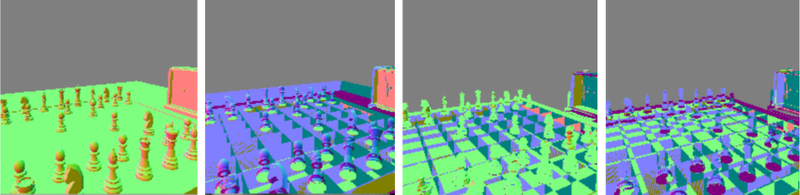

– 4x Depth-peeled layers, without backface culling, showing the surface normals as RGB

Instead, since RTX is not available in WebGPU, this renderer uses a “layered depth image” instead of a K-D tree or other 3D structure. The scene is rendered from a camera to find the closest surface at each pixel, using a standard GPU rasterization pass. We then render successive depth layers by “peeling” them away using the depth at the previous layer. We store the depth, normal, color and other surface properties for each pixel in what is called a G-Buffer. (“G” stands for “geometry” and other well-known algorithms already created Z-Buffers, or, like one of our early film renderers at PDI, an improved A-Buffer.) The downside to this approach is that you only can intersect with objects that you see from the camera. There are ways to mitigate this, like rendering a larger viewport, or multiple views, but they don’t fix the core nature of the screen-spaced intersector.

The current implementation starts with a 4-layer depth peeled GBuffer that stores the linear view space depth, the normal, color, material, and velocity at each layer. Then we create a hierarchical ZBuffer using the depth layer and give all of that to a pass that computes screen-space global illumination (SSGI) by generating one or more ray sample paths using a physically-based PBR material modeled using GGX and cosine sampling patterns. The energy-conserving collection of results is then given to a Spatial-Temporal Variance-Guided Filter (SVGF) which uses a ton of heuristics to collect samples over time to smooth out the noisy MIS samples. The samples use a Heitz Randomized Quasi Monte-Carlo (RQMC) sampling pattern that devolves to blue noise to further minimize noise. The final HDR result is then passed through an ACES tone mapping pass and gamma corrected for final display. A total of five passes, though the GBuffer pass requires rendering the geometry four times, once for each layer. The other four passes are screen-space, one fragment per pixel passes.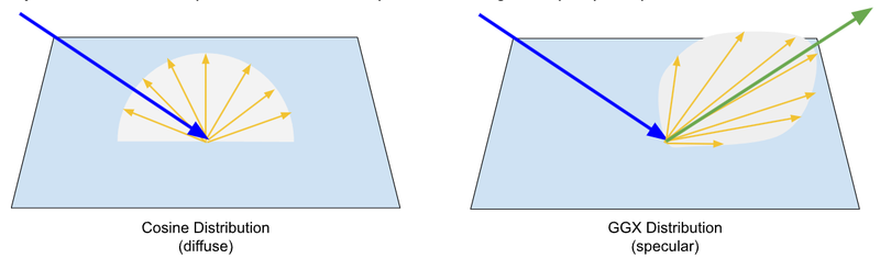

– GGX sampling prioritizes the reflection direction, widening with roughness, and cosine sampling is uniform in all directions, even behind the incident ray.

The MIS sampling has several modes, importance sampling of the HDRI environment map, GGX sampling of the two-layer clear-coated PBR material, cosine sampling for pure diffuse surfaces. The importance sampling uses a Cumulative Distribution Function, which feels like a fancy “Summed Area Table” from the old days to place more samples at bright points in the environment map to reduce noise.

The SVGF filtering tries to accumulate up multiple samples by averaging the frames over time. It has heuristics which look for moving geometry and changing illumination to reject the history samples, which leads to the “ghosting” artifacts you can see when dragging pieces.

All of these passes are implemented as WebGPU fragment shaders, with token vertex shaders in most cases. A total of 4000 lines of WGSL code, with about half of it in the SSGI tracing, which includes all the MIS sampling and HZB DDA ray tracing.

Hierarchical ZBuffer DDA

The inner loop of the SSGI pass traces rays through the GBuffer, accelerating long rays using the hierarchical ZBuffer to skip over large areas of empty space. Most of the scene is empty space, and even with a fast full-resolution ray-walking DDA (Digital Differential Analyzler), which steps along all the pixels touched by a ray in the GBuffer, spends the vast majority of its time stepping through empty space with no intersections.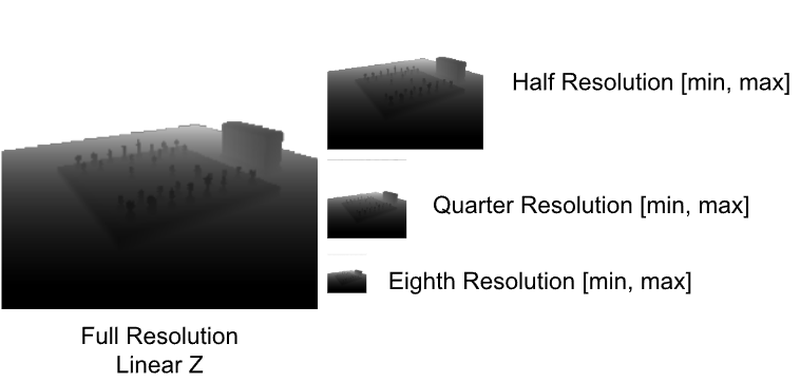

– A hierarchical Z-Buffer stores the min and max Z value from the four pixels in the finer parent level

Stepping our ray through coarser levels of the HZB allows us to skip over empty space many times faster. Our algorithm starts at the finest level, and ascends to a coarser level after three steps without intersections. Any intersection causes it to descend to a finer level until it reaches the finest resolution GBuffer, where we intersect the ray against the two objects represented in the 4-layer GBuffer ([0,1] are the front and back of the first object, and [2,3] are the second object, remember no backface culling).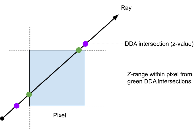

– The DDA stepper returns the z-value at each intersection with a pixel edge during the walk, allowing us to compute the z-range

To properly intersect the ray with the depth values in the GBuffer, we need to know the Z-range of the ray within the pixel. Fortunately, a good DDA provides exactly these values, along with the ability to take a step forward along the ray using fast addition operations, returning the next ray-to-pixel intersection points and their corresponding depths in view space. Given the z-range of the ray within the current pixel, we can compare that against the depths in the GBuffer. In fact, since we render the GBuffer with face culling disabled, we know the boundary representation objects we draw will have the range of z-depth in the depth layers 0 & 1, and then the next two front and back faces in indices 2 & 3 of the GBuffer layers. This gives us two ranges to compare, the ray and the occluding surfaces in the GBuffer, so we can perform exact intersections and interpolate the surface properties between the front and back surface at the ray intersection point.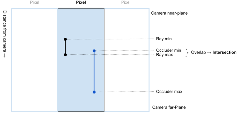

– Looking down on three adjacent pixels, with the camera at the top, showing the ray and object z-ranges used for intersection

When we construct the Hierarchical ZBuffer (HZB), we maintain the four view-space linear Z values in the single output fp32 RGBA 4-tuple by computing the min and max z-value from the input depth values. This allows us to do the same comparison at each level in the HZB using a z-range at each level. The conservative HZB merely accelerates over empty space, and we descend all the way down to the full-resolution GBuffer to perform the final intersections, which amounts to about 1.2 times per pixel, in our chess board scene.

Fast Path

When I first released the app, the fastest rendering path used one path sample per pixel, and perhaps reduced the maximum ray length and number of bounces. Unfortunately, this is still too slow for the vast majority of the general population. It was a bit too frustrating that I had to add a big disclaimer about the required hardware. So, I decided to add a fast path that should be able to still do a reasonable job of approximating global illumination using a fast screen-space ambient-occlusion approximation called XeGTAO (Ground Truth Ambient Occlusion from the Intel XE team).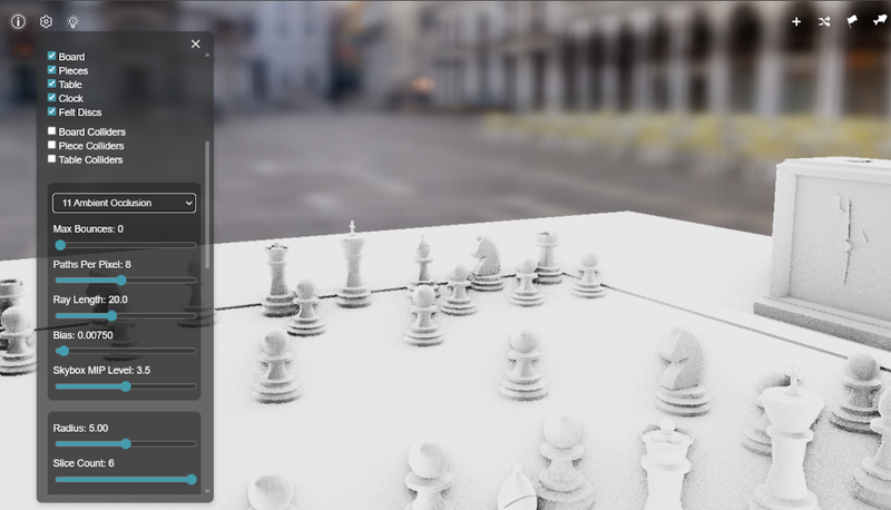

This fast path is now automatically selected based on the calculated frame rate. In fact, the frame rate is used to dynamically adjust all of the rendering quality levels, down to the XeGTAO fast with and up through full multi-bounce path tracing, increasing the number of paths sent per pixel per frame.

We can also improve the quality of the fast path, with only a minor hit to performance, by using the computed AO to approximate ray tracing in any given direction from a surface in our AO texture. This means we approximate the ray intersection with a single lookup in the AO texture. This may allow us to approximate multiple paths per pixel in a single pass, and still be faster than a single full ray trace.

Next Steps

Adding refraction and transparent surfaces is next on the rendering TODO list. It can use the existing ray tracing logic. This will allow us to add the clear glass face on the chess clock as well as adding glass pieces and boards. It will require a slight refactor of the GBuffer layout to include the material ID and UV so that we can re-interpolate the surface textures, since we’re full up and cannot easily add the transparency and index of refraction components without this refactor.

The core flaw of this GBuffer-based approach is the screen-space limitation for occluders. One easy improvement is to pad the boundary of the rendered image, which mitigates these sorts of artifacts. Or, we could even render multiple cameras, to compute a hemisphere or full cube map around the camera.

Finally, due to technical complexities in the SVGF velocity and edge calculations, I had to remove the subpixel camera jitter which would normally be making the geometric edges, like on the chess clock and the edge of the board and piece silhouettes, much smoother. I could enable MSAA, but I’d rather dive in and really enable normal jitter, since it fits in so nicely with the path tracing.

---

Please join my 3D Chessboard Discord server to chat with me directly. Try out the 3D Chessboard online. It's free!